Better Reliability Predictions Using Experience Data
There are many approaches that can be used to predict the reliability of an item. Sometimes when asked to provide a “quick estimate” of an item’s reliability, the use of field experience is overlooked, or if no failures have occurred, overly conservative estimates are made by assuming one failure. This article describes a simple approach for making reliability estimates from limited experience data with no failures, or conversely, answering the question of how much failure-free experience data is required to demonstrate some level of MTBF.
MTBF Calculation From Field Data
Many companies that make use of commercial-off-the-shelf (COTS) items in their system integration process face the task of making reliability estimates for these items based on limited knowledge. These estimates are often needed to feed into some overall system model or to be compared to some reliability allocations. Although generic handbook failure rate models such as those published in MIL-HDBK-217, “Reliability Prediction of Electronic Equipment,” could be used, they require a detailed parts list and many labor hours to develop a failure rate prediction. An easier and more accurate approach (if significant experience time exists), is to calculate a mean-time-between-failure (MTBF) based on field and/or test experience data from identical or similar items.
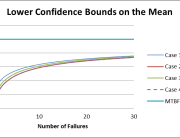
For example, lets say that a notebook computer were being integrated into a larger system and a reliability estimate was needed for this item. No reliability data could be obtained from the notebook manufacturer; however, two similar notebook computers were in continuous use for the previous year with no failures occurring. Using this limited information, the MTBF can be estimated as follows. The total experience time on the two notebook computers is 17,520 hours (2 computers * 1 year * 8760 Hr./Yr. = 17,520 hours). If one failure is arbitrarily assumed, the point estimate of the MTBF is simply 17,520 hours. This approach results in a conservative estimate because it assumes that one failure has occurred when none has. A better approach is to make use of the chi-square distribution for calculating confidence levels for time truncated tests with zero failures occurring. The chi-square distribution can be used to calculate upper and lower confidence intervals for systems that exhibit a constant failure rate (i.e., exponential failure distribution), as commonly observed with complex electronic systems. When zero failures have occurred, it is common to calculate the lower 60% confidence level for MTBF.
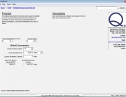
The Quanterion Automated Reliability Toolkit (QuART) provides a quick and easy way to make this calculation. As shown in Figure 1, simply select the time-truncated test option, enter the experience time, the number of failures and the confidence level desired. For this example, it can stated with 60% confidence that the MTBF of a notebook computer is at least 19,121 hours.
MTBF Demonstration Test Length
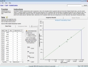
A related question that often arises is “how much experience time with zero failures is needed to prove some level of MTBF?” For example, if the allocated reliability for the notebook computer above were 30,000 hours, how many failure free experience-hours would need to be accumulated to prove that the allocated MTBF was achieved with a high degree of confidence (e.g., say 90%)? Using the QuART confidence level calculation tool, simply select time-truncated test option, enter 90% for the confidence level, and through several trial and error guesses, the time required is found to be 69,078 hours, as shown in Figure 2. Therefore, eight computers (69,078 hours / 8,760 Hr./Yr. = 7.9) would need to run failure free for almost one year to prove that a 30,000 hour MTBF requirement was met with 90% confidence.

Figure 1 – MTBF Estimate with Zero Failures
Figure 2 – Test Time Required to Demonstrate an MTBF
Significant Experience
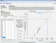
The above approach requires some judgment as to whether or not accumulated time is “significant,” otherwise extremely pessimistic MTBF estimates can be calculated. For example, if the item under consideration above were a single device, say a microcircuit, accumulating 17,502 experience-hours would be considered “insignificant” since other sources (e.g., MIL-HDBK-217, Telcordia SR-332, etc.) indicate that the MTBFs for microcircuits are on the order of tens of millions of hours, not tens of thousands. Therefore, a “ballpark” estimate/guess of the expected MTBF is often helpful in making a judgment as to how much experience-time is “enough time” for making realistic MTBF estimates. One tool for making this judgment is the QuART Reliability Potential Calculator. This tool requires only an estimate of the number of parts in an item, its use environment, and an assumed part quality level to provide a ballpark MTBF estimate. For example, if we guessed that a notebook computer consisted of 1000 commercial quality parts operated in a ground benign environment, the QuART Reliability Potential tool estimates a ballpark MTBF (based on MIL-HDBK-217 relationships) of about 6300 hours, as shown in Figure 3. Therefore, accumulating several multiples of this time (17,500 hours) on the two notebook computers would be viewed as “significant” experience time.
Figure 3 – QuART “Reliability Potential” Estimate